

The study of gull identification has come so far that many of the questions at the forefront require blood tests and whole-genome sequencing to yield satisfying answers. Yet this does not stop people from posing these questions to birdwatchers as if one could learn the answers through experience in the field. Questions of “hybrid” vs. “pure” ancestry, subspecies distinctions in the Iceland Gull complex, and juveniles in the Herring complex (American, European, Vega) are just some of the cases where birds often defy our attempts to confidently categorize them based on appearance alone.
As birdwatchers, we really want to know where birds are from: is that a vagrant from another continent sitting in front of me, or just a weird Herring Gull? You know that both are possible. You remember that adult Black-tailed Gull sitting on the same beach last summer. What people often don’t realize is that when gulls show complete overlap in appearance, or when the boundaries between taxa are unclear, the question of origin necessarily becomes a question of genetics.
In what follows, I will first give an objective description of what it is we are doing when we sort through gulls with field marks, and then I’ll show why this approach falls short when dealing with an unknown degree of overlap. I’m using a thought experiment I call the “Perfect Vagrant,” which depicts a scenario I have seen played out over and over again when people turn up candidates for rare gulls. In a nutshell, the Perfect Vagrant Fallacy is the idea that by identifying enough traits with average differences, there exists some “tipping point” around which individuals can be placed in one or another taxa. From there, I will examine a range of processes that can create overlap or blur the boundaries between species. These mechanisms are neither speculative nor rare; they are likely influencing gulls today or shaped their ancestors in the recent past. While some of these topics might seem tedious (when is a group a “subspecies” rather than a “species”?), even a limited understanding will begin to reveal the true nature of the questions at the forefront in gulls.
Though we may not always get satisfying answers when it comes to the origins of a bird, this does not mean the study of these birds is over, even for someone armed with a pair of binoculars and a camera. There is still so much to learn from these “problem” birds if we first accept that we might have to deal with appearances only, at least at first. The details and relationships of observable traits are interesting in their own right, but the information they offer can also steer the course for genetic research. After all, if genetic research is going to be meaningfully related to what we can observe, it is first necessary to accurately describe what we observe.
Gull-watchers are statisticians
Here’s a familiar story for gull-watchers on Lake Michigan. You scan through a flock of Herring Gulls until you land on an adult bird with smudgy brown marks on its head and neck. The bird has a somewhat smaller bill and head, but not super small, and it has a dusky iris. Could this be a Thayer’s-type Iceland? The wingtip is very similar to the Herrings nearby, so that would be a dark wingtip for Thayer’s…

What is happening in your head? Our instinct when dealing with two types of gulls that have overlapping traits is to look for the traits that have average differences, then to compare the likelihoods that the combination of traits we observe would appear in an individual of either type. For the example above, this looks something like this:

What happens in our heads is literally a multiplication problem: we search through our mental samples for each species, coming up with likelihoods for each trait we are seeing. The way probabilities work, it is the product of each trait’s likelihood that gives the likelihood that all of those traits will occur at the same time in a single individual. It is by comparing the ultimate likelihoods of each species, i.e. creating a relative likelihood, that we arrive at an identification. As we pile on more traits, the likelihood of a bird belonging to one species hopefully shrinks to near zero, leaving the other species as the safe option. If you see the wingtip of the bird above and it has contrasting pale inner webs on the primaries, the likelihood it is a Herring shrinks considerably. If you see a bright pink orbital, the likelihood of this in Herring is theoretically zero–a so-called “hard” field mark–and you can seal the deal on Thayer’s.
Also entering into your mental arithmetic is the expected frequency of each species at that location. If this would be a country’s first record of a Thayer’s, you might want to see an open wing or orbital before you “call it.” On the Great Lakes, where Thayer’s types are expected at a certain frequency, someone might feel comfortable calling a bird without seeing every definitive trait. Running the same program with Glaucous-winged x Herring hybrid instead of Herring Gull would yield yet another result, again with different likelihoods depending on the location.
The likelihoods of traits and the accuracy of mental samples are what we gain with experience. It is the seasoned gull-watcher who has been fooled by that 1/1000 Herring Gull so many times who is more hesitant to call a bird a Thayer’s; the same person might “magically” pick out a solid Thayer’s in the back of the flock by recognizing the right combination of traits that are obscure to others. While experience can allow people to become magicians with Herrings and Thayer’s, there are limitations when you come to groups that have more extensive overlap or blurred boundaries.
The Answer to the Thayer’s vs. Kumlien’s Question
Just kidding! Instead, here’s a deeper dive into statistics. The Iceland Gull complex offers a great example of how people have changed their perspective of traits as more understanding has been gained. (Acknowledging the uncertainties involved in The Iceland Gulls–more on that later–I will be using “Thayer’s” and “Kumlien’s” designations for simplicity and congruence with previous work).
Three studies in the late 1990s and early 2000s created a scoring system and measured iris coloration of wintering Thayer’s Gulls in California and Kumlien’s Gulls in Newfoundland. Here’s what they found:

Combined data from King and Howell (1999) and Howell and Elliot (2001).

Data from Howell and Mactavish 2003. Of note, the authors state “darker-eyed Kumlien’s Gulls than those in our sample do occur (pers. obs.).”
These two bar graphs, overlaid and approximated as smooth curves, look something like this:

Prior to these studies, references supposedly portrayed Thayer’s Gulls with dark irises and Kumlien’s Gulls with pale irises, without acknowledging overlap. With these studies, including the part where the authors say, “there are Kumlien’s out there with darker irises than ours,” it was shown that there could very well be complete overlap of iris coloration in Thayer’s and Kumlien’s types wintering on opposite sides of the continent. So, is iris coloration at all useful for distinguishing Thayer’s and Kumlien’s types?
Take a look at some of the measures that arise from these trait distributions.

Range is pretty familiar to gull-watchers. Questions like, “Is this trait within range?” are common enough. In the case of iris coloration in Thayer’s and Kumlien’s, looking at the ranges alone does not lead to any significant differences between the sample groups (the “?” in Kumlien’s is safe to remove now but kept here to represent the sample in this study).

Adding in the frequencies (the vertical axis) of each score in the two samples adds another dimension to the range. While old references were misleading in not acknowledging overlap in iris coloration, the decision to portray Thayer’s with dark irises and Kumlien’s with pale irises was not random; it was based on real average differences. The type of average shown here is the “mode,” referring to the single score shared by the largest number of individuals in each sample. You can see the curves intersect somewhere around the score 2. This means, when considering iris coloration alone, any individual with a score above 2 is more likely to be found in the Kumlien’s sample, while scores below 2 are more likely to be found in the Thayer’s sample. This gives iris score some predictive power, but you may still be skeptical, and for good reason.

Variance describes how closely the scores in a sample cluster around the mean (if you assume the above curves are symmetric, which they sort of are, then the mean is equal to the mode, i.e. the score at the peak of the curve). In these studies, iris scores in the Thayer’s sample have an appreciably higher variance than the scores in the Kumlien’s sample. Another way to conceive of variance is to imagine how difficult it would be to recognize a “typical” appearance of a trait from experience. In the Kumlien’s sample, almost 60% of individuals had the same score of 2.5. It is realistic to assume you might recognize a “typical” iris after spending time with Kumlien’s. Contrast this with the Thayer’s sample, where the iris scores are much more spread out. Even though there is an average, it might be hard to put your finger what that average is without looking at a graph.

The graph on the right shows an imaginary case where the Thayer’s distribution has the same range and mode, but a much lower variance. For the iris score of 2.5, shown with the dashed line, you can see how a different variance greatly affects the relative likelihood that this iris score can be found in each sample. The iris score of 2.5 is about 4x more likely to be found in Kumlien’s in the actual case (60%:15%), and about 12x more likely to be found in Kumlien’s in the imaginary, low variance case (60%:5%). That’s a threefold difference in relative likelihood, only from altering the variance, while keeping the ranges and averages exactly the same. Remember, it is these relative likelihoods that we are interested in when we are sussing out field marks in the real world.
Multiple traits
It’s likely that people can form fairly accurate impressions of range, average, and even variance with enough experience. Taking measurements and creating trait distributions like this can certainly lead to more accurate estimations of likelihoods, but things get really interesting when multiple traits are considered. This is due to the possibility of covariance. When traits covary, that means that a variation in one trait is more likely to occur along with a particular variation in another trait. Going back to the potential Thayer’s scenario, if smudgy heads and dark irises are known to covary in Herring Gulls, then this makes the occurrence of these two unlikely traits more expected if they occur together in the same individual. Like variance, covariance of multiple traits can greatly alter the ultimate likelihoods of trait combinations.


Common Redpoll (left) and Hoary Redpoll (right) “ecotypes.” Photo credit: Seabrooke Leckie/Flickr Creative Commons.
Birdwatchers had long recognized that bill size and plumage darkness covary in redpolls when researchers discovered that genes associated with these traits are usually linked; these genes are physically connected on a relatively small stretch of chromosome and inherited as a unit.
While people might be able to pick up on two or three traits that seem to change together, when more traits are added in, it seems doubtful that humans are capable of discerning all of the possible covariances without analyzing measurements. Being unaware of covarying traits is just one way to end up with inaccurate estimates of relative likelihoods, and this is still only considering appearances.
Now consider what happens when this pattern of thinking is applied to a case with multiple traits that show complete overlap.
Trash Bird vs. Mega Rarity - The “Perfect Vagrant”
Imagine two gull species called “Trash Bird” and “Mega Rarity.” You live in a location where Trash Birds are very common, whereas a Mega Rarity would be, well, a mega rarity. A Mega Rarity is not like a Thayer’s type on the Great Lakes, but more like a Thayer’s on the East Coast or in Europe. You find an interesting candidate one day in your local patch, a juvenile, call it “Bird X,” and you’d like to know if Bird X is a Trash Bird or Mega Rarity.
Fortunately, researchers have studied representative samples of known populations for each species in their expected range. Unfortunately, the only traits known to show differences in these species as juveniles just show average differences; there are no field marks that are exclusive to one or the other species.
The blue and red curves below represent the scores determined by the researchers for each trait in the two species–these are just like the curves for Thayer’s and Kumlien’s in the previous section. Bird X’s specific score for each trait is shown with a green dashed line.
(Before going on, it’s worth mentioning that there are many possible complexities in the shapes of bell curves. These complexities are being ignored for the sake of a thought experiment. The curves below are “real enough” to make the point.)

For three traits, Bird X looks very much like a typical Mega Rarity, with iris coloration particularly “Mega-leaning.” Bird X’s wingtip darkness, however, looks more like a typical Trash Bird. What can you say about Bird X in this case?
Response 1 - “Trait 1, Trait 2, Trait 3… you’ve got it! A Mega Rarity!”
This is one version of what I am calling the “Perfect Vagrant Fallacy”: very few if any Mega Rarities are “perfect” in their expected range. After all, Mega Rarities are gulls; they are variable. Bird X would not stand out for a second in a flock of Mega Rarities, while this particular combination of “Mega-like” traits in a Trash Bird would simply be too much of a coincidence. Thus, Bird X is safely labeled as a Mega Rarity.
The problem with Response 1: This pattern of thinking, while it works well with Thayer’s and Herring Gulls, falls apart when there is complete overlap in traits and the frequency of vagrancy is unknown. Stated another way, this response is saying that the probability of a Mega Rarity showing these traits and turning up as a vagrant is higher than the probability of a Trash Bird showing these traits in its expected range. While it is possible to estimate such probabilities, for these estimates to be meaningfully accurate requires some key pieces of information–and as I’ll discuss, that information is often lacking.
Response 2 - “Close, but Trait 4 looks like a Trash Bird. Given your location, this is most likely an odd Trash Bird.”
This is another, more familiar, version of the “Perfect Vagrant Fallacy”: Bird X is close to being a Mega Rarity, but it’s not perfect, and Mega Rarities should be held to a higher standard outside of their normal range.
The problem with Response 2: while this “all or nothing” reasoning may seem more conservative, it is subject to the same caveats as Response 1. Stated another way, this response is saying that the probability of a Trash Bird showing these traits in its expected range is higher than the probability of a Mega Rarity showing these traits and turning up as a vagrant. Again, estimating these probabilities is possible, but these estimations usually involve too many unknowns to be meaningfully accurate.
Response 3 - “A lot of these traits resemble Mega Rarities, but a Trash Bird cannot be ruled out.”
This is better. For one, it is true.
The problem with Response 3: I have no serious gripe here. You’ll notice that this response does not claim which option is more likely without supporting evidence. My only minor complaint is that the person hearing this is likely to lump Bird X into a garbage bag with countless others, the so-called “Good Candidates.” What if there is something meaningful about the particular combination of traits shown by Bird X? Is there some pattern shown by other individuals? While this response is not problematic, throwing away cases like Bird X may be missing the opportunity to learn something.
Response 4 - "Mega Rarities are about 3 times more likely to show this combination of traits than Trash Birds. Even so, this individual is likely to have originated from a northern population of Trash Birds that retains Mega-traits due to hybridization and introgression that occurred during the last glacial maximum around 20,000 years ago."
A bit extra? What I’ve tried to do here is come up with a hypothetical response that could draw on any potential research a person could ask for short of a name tag on Bird X itself. Data for each species could include trait distributions, whole genome sequencing studies, maybe a big database of geolocator recoveries. Even with all this data, there is still the possibility that Bird X might have just a “slight” probability favoring one species over the other, or it could even turn out to be ambiguous.
What is the likelihood of vagrancy?
Even if people obtain representative trait distributions in a species, and they check for the possibility of covarying traits, this still only gives the likelihood that an individual will show a certain appearance in the expected range of that species, or wherever such a sample was created. It says nothing about the likelihood that an individual of that species will occur at a different location. The likelihood of vagrancy is extremely difficult to estimate with any precision, as gulls can be highly unpredictable (that’s part of what makes them so fun!). Gulls turn up in new and unexpected locations all the time. This can be due to increased observer coverage, broad patterns of change in distribution, or simply some individual gulls with a propensity to wander.
This unpredictability can lead people to ignore the likelihood of vagrancy altogether. When broader patterns emerge, biases can creep in. For example, with vagrant Slaty-backed and Vega Gull sightings on the rise, should we expect a significant proportion of these vagrants to be juveniles? Is the abundance of adult records due to their more distinct appearance, making them easier to identify, or does it reflect real differences in vagrancy patterns across age groups? Could juvenile vagrants be even more frequent than adults? It’s probably not safe to assume the answers to these questions. Banding recoveries, geolocator studies, and increasing long-term field observations can offer some insights, even if these are incomplete.
What is the likelihood of overlap?
In reality, trait distributions like those illustrated above have rarely been measured. Instead, they are estimated from the study of appearances. This often leaves a gray zone at the tail ends of distributions, leaving the degree of overlap between groups unknown. In cases like Bird X, this forces people to weigh two uncertainties: the likelihood of vagrancy, which is highly imprecise, versus the likelihood of trait overlap between the species or types in question. In order to bring the gray zone of distributions into focus, it really requires an understanding of the genetics involved when defining different groups.
To see why, the following sections explore mechanisms that drive overlap between groups like Trash Bird and Mega Rarity. Down one path, the validity of treating any two groups as distinct species in the first place is called into question. Down another, if species (or subspecies) designations hold up, there is still the possibility that the evolutionary history between groups can lead to overlapping appearances in modern times.
A basic understanding of genetics and common ancestry will be helpful for the next sections. You can learn or refresh these concepts through the following YouTube videos:
Some ways a bird can look like a Mega without being from Megaland
Gene flow in the recent past and present: hybridization, introgression, and the emergence of “types”
If Trash Birds and Mega Rarities overlap in range and produce hybrids, and those hybrids can then breed and produce offspring with individuals of either parent species, this creates a scenario where genes and traits can be passed between species. This is called introgression, and it is a form of gene flow, as the genetic variation from one group can “flow” into another group. With more gene flow, the genetic distinctiveness between groups diminishes. In general, different species have a lot of genetic distinctiveness (lower gene flow), while different subspecies in the same complex are less genetically distinct (higher gene flow).
One interesting consequence of introgression is that the observable traits in an individual, called its phenotype, might not always associate with its genetic variation, called its genotype, in an obvious way. For example, in a study of the Glaucous Gull-European Herring Gull hybrid complex in Iceland, researchers found that some hybrid individuals with appearances most resembling Glaucous Gulls could have genetic markers more in common with Herring Gulls. Likewise, some individuals that appeared to be “pure” showed genetic markers of both species, i.e. hybrid ancestry. When introgression is extensive, you cannot infer an individual’s genetic ancestry based solely on its appearance–including assumptions of “purity.”
This is a key understanding that people are missing on a daily basis in online gull forums. Statements like “this looks good for a pure Glaucous Gull” are really saying that a gull looks like most Glaucous Gulls, not that it necessarily doesn’t have hybrid ancestry.

Glaucous x European Herring hybrid. 04 August 2024. Reykjavik, Iceland. While the individual above most closely resembles a Glaucous Gull in appearance, genetic research on this complex found that a portion of “Glaucous-leaning” hybrids showed genetic markers more similar to European Herring Gulls due to introgression.
Things get really interesting when you compare how phenotypes vary to how genotypes vary. As observable traits are on some level necessarily associated with genes, you might expect that distinct groups of individuals based on phenotype show similarly distinct genetic variation. However, modern research with whole-genome sequencing is revealing more and more cases where groups that show obvious differences in phenotype show surprisingly little difference genetically; often the genetic differences involved are so minute that they likely require whole-genome sequencing to detect at all. In these cases, the term “type” has often been used to describe these observably distinct groups that nonetheless show largely similar genomes, e.g. “morphotype” or “ecotype.”

Illustrations of different patterns of variation in populations. (a) Depicts a sharp categorical break, (b) a gradient with two strong clusters, (c) a continuous gradient with no clear clustering, and (d) uniformity. While (a) through (c) all contain the recognizable extremes of “black” and “white,” statistically significant clusters only exist in (a) and (b).
The degree to which two birds are “different,” whether in their observable traits or their genomes, can be measured and described statistically. These differences can then be assessed across a population to determine whether distinct groupings have statistical strength, an attribute known as population structure. There may be two strong groups, three, more, or none at all. Whether these groups warrant labels such as “species,” “subspecies,” or “parent and hybrid” should emerge from the statistical patterns of variation within the gene pool rather than being assumed beforehand. The details of the statistical methods used, such as clustering algorithms, are beyond the scope covered here, but if modern research in this field has taught us one thing, it is not to assume that the patterns we observe in phenotypes will be similarly reflected in genotypes.
This last point is especially relevant with large white-headed gulls, as genetic research to date has shown that recent gene flow between these taxa is extremely prevalent, and it leads to a key uncertainty in the “Perfect Vagrant” scenario: if there is an unknown degree of gene flow between Trash Birds and Mega Rarities, then the two may not form genetically distinct groups–even if such groups exist, how phenotypes associate with each group may not be obvious. Even if Trash Birds and Mega Rarities each hold a high degree of unique genetic variation typical of species or subspecies, if there is extensive introgression between the groups, then appearances may be deceiving. In regards to geographic origin, it is likewise not fair to assume that intermediate-looking hybrid types will always originate in a clearly defined “hybrid zone.”
Below are three examples where whole-genome sequencing has revealed surprisingly little genetic differentiation in complexes where phenotypes show sizeable variation. In these cases, the attributes of phenotype, genotype, and geographic origin combine in different and sometimes unexpected ways, demonstrating that the pattern in one realm does not always imply the same pattern in another.
Northern Flicker complex

Source: Aguillon, S. M., Walsh, J., & Lovette, I. J. (2021). Extensive hybridization reveals multiple coloration genes underlying a complex plumage phenotype.
Phenotype. Traits group together strongly in ranges of two parent types and mix in various combinations in hybrid zone where parent ranges overlap. Variation in traits across hybrid types may occur in more distinct steps with few intermediates, e.g. trait #6, or in more subtle gradations, e.g. trait #3 and #5.
Genotype. Genome-wide genetic variation weakly correlates with phenotypic scores on a gradual cline. Genetic variation does not clearly distinguish between parent and hybrid phenotypes in every case. For example, some red-shafted individuals may share more genetic variation with some hybrid type individuals than with other red-shafted individuals. Gene flow between parent types is relatively high compared to other taxa considered “subspecies.” Fixed differences unique to each parent type account for only 0.011% of total genomic variation (780 fixed SNPs in parent types out of 7.25 million SNPs in the entire sample of parent and hybrid types).
Geography. Parent types mostly originate in different ranges, with overlapping range producing hybrid types. Identification of hybrid types and placing their origin is straightforward in some cases due to the discrete nature of traits, e.g. malar and crown coloration. In other cases, hybrid ancestry will be less obvious due to traits that show gradual variation, e.g. subtle gradations in red to orange coloration in tail and flight feathers. In yet other cases, hybrid ancestry may be completely masked by parent-type traits, e.g. a red-shafted type with hybrid ancestry. Possible recent changes to boundaries of hybrid zone.
Blue-winged x Golden-winged Warbler complex

Source: Toews, D. P. L., S. A. Taylor, R. Vallender, A. Brelsford, B. G. Butcher, P. W. Messer, and I. J. Lovette. 2016. Plumage genes and little else distinguish the genomes of hybridizing warblers.
Phenotype. Traits group strongly in ranges of two parent types, mixing in various combinations in hybrid zones. Variation in some traits usually occurs in more discrete steps, e.g. throat pattern in males, while others vary more gradually, e.g. wingbar coloration.
Genotype. Six small genomic regions account for most phenotypic variation, with four of these regions near genes associated with feather development or pigmentation. Details of how variations in these genes relate to transitions in phenotypes are not fully understood. The rest of the genome shows no significant correlation with phenotype. As a result, the phenotype of an individual says nothing about the phenotypes of its closest relatives in the complex.
Geography. Similar to flickers. Parent types generally breed in different ranges, with hybrid types originating where their ranges overlap. Identifying individuals with hybrid ancestry and placing their likely origins in hybrid zones may be straightforward in cases with obviously intermediate phenotypes, difficult in cases with subtle gradations in traits, or impossible when hybrid ancestry is completely hidden behind “pure” parent phenotypes.
Redpoll complex

Sources:
Mason, N. A., and S. A. Taylor. 2015. Differentially expressed genes match bill morphology and plumage despite largely undifferentiated genomes in a Holarctic songbird.
Funk, E. R., N. A. Mason, S. Pálsson, T. Albrecht, J. A. Johnson, and S. A. Taylor. 2021. A supergene underlies linked variation in color and morphology in a Holarctic songbird.
Phenotype. Plumage and bill size vary, tending toward two extremes—one with paler plumage and smaller bills (Hoary-end), the other with darker plumage and larger bills (Common-end). Traits appear to vary along continuous gradients, with a full range of intermediates and no obvious breaks in variation. Earlier scoring systems were based on observed range of variation in traits assumed to covary, with no quantitative analyses of the strength of covariance or statistical tests to assess trait clustering.
Genotype. Different phenotypes are most likely traced to a single chromosome with a stretch of DNA that may be inverted (literally flipped backwards) or not. An individual with two copies of the inversion correlates to one type, two copies without the inversion to the other type, and heterozygotes (one chromosome with the inversion, one without) correlates to intermediate traits. The gradual variation in phenotype is suspected to arise from different rates of expression in this inversion region. How these three genetic variants connect to phenotypes on a finer scale is not understood, e.g. the classical understandings of “Hoary” vs. “Common” types and previous scoring systems. The genomes outside of the inversion site show no significant differences across the complex. An individual’s phenotype provides no clue as to the phenotype of its closest genetic relatives in the complex.
Geography. Hoary types tend to breed at higher latitudes than Common types, with heterzygote individuals showing an intermediate trend with latitude. Extensive overlap in breeding ranges exists between different types, with no well defined “hybrid zone.” Discriminating the potential origins of individuals based on different phenotypes is not possible outside of broad trends in latitude, e.g. a Hoary type is less likely to originate in more southerly latitudes.
It’s worth taking a minute to consider how the aspects of phenotype, genotype, and geographic origins occur in the cases above in terms of different patterns of variation.

Illustrations of different patterns of variation in populations, often referred to as population structure. (a) Depicts a sharp categorical break, (b) a gradient with two strong clusters, (c) a continuous gradient with no clear clustering, and (d) uniformity. While (a) through (c) all contain the recognizable extremes of “black” and “white,” statistically significant clusters only exist in (a) and (b).
Across the redpoll complex, variation in individual traits or combinations of traits resembles c), while the genetic variation associated with those traits resembles a), and genetic variation across entire genomes most resembles d). Across the flicker complex, variation in phenotype can resemble b) for certain traits, c) for other traits, while genetic variation across the genome is somewhere between c) and d) (but much closer to d)).
These illustrations can also be loosely applied to geographic origins. In flickers and Vermivora warblers, intermediate types are most likely to originate within well-defined hybrid zones, with parent types dominating outside of them—similar to pattern b). In redpolls, however, the probability of an individual’s geographic origin follows a latitudinal gradient, with no distinct hybrid zone—more like pattern c).
What happened to the Hoary Redpoll?
The form once referred to as the “Hoary Redpoll” turned out to be generally related to a very concrete group based on genetic variation, only the actual genetic differences involved are shockingly small. The group is nowhere near what is typically considered a “species” or a “subspecies,” but it is a clear and well-defined genetic group nonetheless. That said, no one has yet demonstrated how statistically distinct this genetic group is based on appearance. Researchers used an arbitrary classification system to sort individuals into phenotypic categories, much like the ones birdwatchers used to rely on, yet this system worked well enough and revealed strong correlations to different genotypes, which is really what the researchers were after. So there exists a group of genetically distinct Hoary Redpolls out there, and they look different, but whether this group shows defined boundaries in appearance, or if it would be at all practical for birdwatchers to recognize such boundaries, is just as unclear as it ever was. Ironically, different scoring systems like the ones used in the past can actually be tested now, yet discussions on redpoll classification seem to have mysteriously ceased following the redpoll lump into a single species…
Now consider the Iceland Gull complex. We know that variation in traits appears to vary more gradually, with certain combinations of traits suspected to cluster more strongly. With the number of traits involved, the existence of such clusters should ideally arise from measurements and statistical tests rather than experience and intuition. The genetic variation across the complex has not been studied to a meaningful degree. Similarly, the understanding of phenotypic variation across the breeding grounds contains significant gaps, leaving no clear picture of how phenotype relates to geographic origin. The occurrence of traits across the wintering grounds cannot be assumed to reflect the same patterns on the breeding grounds.

A very pale Iceland Gull. Photo credit: Tarik Shahzad. 19 Jan 2025. IL, US.
Answers to questions like "Can this bird be a glaucoides, even though it has faint markings on the wingtip?" depend on how glaucoides as a group varies along the dimensions of phenotype, genotype, and geography. Are you asking whether this bird exhibits a cluster of traits that tend to occur together and rarely in other combinations (phenotype)? Are you asking whether birds with these traits also share genetic similarities distinct from those with different traits (genotype)? Are you asking whether a bird with these traits was most likely born in Greenland (geographic origin)? All are valid questions, but answering them requires statistical analysis of traits and genetic variation, as well as thorough surveying of the breeding grounds–all of which are lacking for the Iceland Gull complex.
Say these gaps in knowledge are someday filled; if enough individuals answer the questions above in alignment, glaucoides might be elevated to species status, while if the answer to one question bears little relation to the answer to another, then the status of glaucoides may be demoted to a “type,” if that.

Attempting to label individuals in the Iceland Gull complex is akin to deciding whether a certain shade in these illustrations is “dark,” “pale,” or “gray.” Such debates frequently overlook the nature of variation involved, even though it is the nature of variation that ultimately determines the meaning and significance of such labels.
Gene flow in the distant past
Introgression that has occurred between two distinct lineages in the distant past, and has since ceased, can still leave traces into modern times.
Imagine a giant chasm opened up in the earth right in the middle of the Olympic Gull hybrid zone. Miraculously, no gulls or humans are harmed. For simplicity, say the gulls to the north of the chasm include all Glaucous-winged Gulls, and the gulls to the south include all Western Gulls, while the hybrids and backcrosses escape randomly to both the north and south. Importantly, the chasm is so large that all of the gulls to the north and south become reproductively isolated. Over time, will intermediate looking “Olympic Gulls” slowly fade out of existence? Not necessarily.
Individuals with intermediate appearances could exist well into the future, even if interbreeding between gulls to the north and south completely ceases. Take the trait of wingtip darkness in the gulls north of the chasm. You might imagine that shortly after the chasm, a first generation hybrid with intermediate dark gray wingtips might backcross with a pale-winged Glaucous-winged Gull, creating offspring with slightly more pale wingtips, and so on into the future, until all the descendants of that hybrid in the distant future ultimately have pale wingtips just like Glaucous-winged Gulls. The genetic variants associated with dark wingtips are gradually diluted and lost. Dark wingtip variants could also be lost due to random events, like natural disasters, or diseases–factors that affect individuals equally regardless of their appearance–but just happen to kill off dark-wingtipped individuals as they probably occurred at a low frequency to begin with. These are examples of genetic drift. Crucially, the dilution of genes and genetic drift can be counteracted by nonrandom selection.
If there are some individuals in the north who happen to prefer mates with dark wingtips for some reason, or if dark wingtips confer some survival advantage, then dark wingtips could persist for some time, even indefinitely; the proportion of northern gulls in the distant future that have dark wingtips will depend on the interplay of these forces. This is not something that is clear-cut or easy to predict. In one scenario, future gull-watchers might consider “Glaucous-winged Gull 2.0” to be a mostly pale-winged species that occasionally shows darker wingtips, even though it does not regularly hybridize with other species and is genetically distinct.

In a hypothetical future where the hybridization of Glaucous-winged Gulls and Western Gulls ceases, intermediate forms such as the gull on the left could still exist well into the future; intermediate traits do not necessarily disappear just because they occur at low frequencies, but could persist depending on the interplay of forces like genetic drift and selection. In one scenario, a reproductively isolated “Glaucous-winged Gull 2.0” could emerge that includes a wider range of wingtip darkness resulting from hybridization in the distant past.
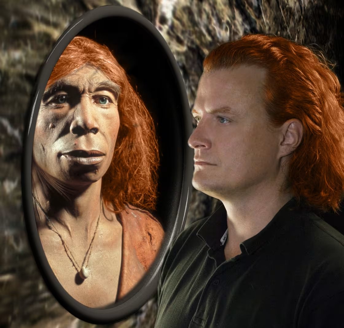
Modern humans and Neanderthals interbred across Eurasia until around 40,000 years ago when Neanderthals went extinct. Most people living outside of Africa today can still trace about 1-2% of their genome to Neanderthals. Why did these genetic variants persist for tens of thousands of years, even after interbreeding ceased? Why did this genetic variation not disappear through dilution with the variants in Homo sapiens or get lost through genetic drift?
Based on the understanding of what traits these genes affect, it is likely the variants conferred selective advantages. For example, some Neanderthal alleles have been linked to lighter skin pigmentation, which may have helped early humans at higher latitudes synthesize more vitamin D from limited sunlight.
Incomplete lineage sorting and founder effect
Incomplete lineage sorting is similar to historic hybridization, with the key difference involving when overlap is introduced in the timeline of lineages diverging from their common ancestors. With historic hybridization, overlap arises from the exchange of genes long after two lineages have split from their common ancestors—there may have been no overlap in a trait before hybridization. In contrast, ILS involves overlap due to genetic variation that existed in the ancestral population, before lineages split.
Say the ancestors shared by both modern day Kumlien’s and glaucoides showed a range of wingtips, from fairly dark to unmarked. These ancestors could split into two lineages, one with mostly darker wingtips, the other with mostly unmarked wingtips, and a small range of overlap between the two. This is incomplete lineage sorting; the way the lineages happened to split makes it seem as if there is ongoing gene flow even though gene flow could have ceased long ago. If only a small subset of the ancestral population split off to colonize a new territory, e.g. Greenland, this could result in a smaller range of variation in the descendants of these “founders” – the founder effect. This small subset could contain some traits that still overlap with the ancestral population and the descendants that remained in the original range.

Incomplete lineage sorting. As two lineages split from their common ancestor, they may contain a degree of overlap. These differences may decrease or disappear over time if descendant populations are reproductively isolated, under different selective pressures, or through genetic drift–or overlap may persist.

Founder effect. A small subset of an ancestral population splits off, maybe to colonize a new territory. The descendants of those in the ancestral homeland may have a large degree of overlap with the descendants of the founders in the new territory.

Past period of hybridization with introgression. Two lineages split from their common ancestor and diverged over time, leading to no overlap in a trait. Then a period of intense introgression introduced novel variations of a trait to either lineage. Even if introgression slows or ceases, overlap can persist for some time. Note that introgression doesn’t necessarily “recreate” ancestral traits that were lost as shown in this simplified scenario.
Background map source: Perrin Remonté
Wingtip illustrations source: The Gull Guide: North America, illustrated by Hans Larsson
The diagrams above are simplified. Selection and genetic drift can create significant change, but these evolutionary forces are removed here to illustrate how each process in isolation can lead to overlap in modern taxa. The backdrop of these diagrams is an artistic rendering of the last glacial maximum, ~20 thousand years ago, when the majority of modern breeding grounds in the Iceland Gull complex were covered by ice sheets (light blue in the map). As glaciers receded and breeding territories expanded, any of these processes could have shaped the ancestors of arctic-breeding gulls, from the emergence of new divisions, to secondary contact between previously isolated groups.
Why do immatures show so much overlap?
Why do adult Vega Gulls look so different from American Herrings while juveniles of these species show so much overlap that some believe it may be impossible to safely identify vagrants? Ditto for Slaty-backed and American Herring Gull, Kamchatka and Short-billed Gull, etc. One answer comes from common descent and the idea that selective pressures vary at different ages.

Top row, left to right: juvenile American Robin, juvenile Eurasian Blackbird. Bottom row, left to right: adult American Robin, adult Eurasian Blackbird. It is probably not a coincidence that the juveniles of these thrushes look so similar; the two species are close relatives, and it’s a good bet that the juveniles of their common ancestors shared some of the same similarities as the juveniles above.
Photo credits, top row, left to right: Paul Fenwick, Josep del Hoyo. Bottom row, left to right: Ryan Schain, Korkut Demirbas
As two lineages diverge from a common ancestor, adults may evolve to look very different while juveniles and immatures remain similar due to different selective pressures acting at different stages of development. In order for this to occur, some genes affecting appearance in juveniles must operate independently from those affecting appearance in adults. We have this to thank for a number of similar (and confusing) immature appearances across the animal kingdom.
Juvenile plumage gives a lot of points for camouflage, which could leave ancestral traits unaltered if surroundings in early life remain similar, a sort of “if it ain’t broke, don’t fix it.” Adults, in contrast, may evolve all sorts of bells and whistles to attract mates and signal to rivals which lead to drastically different appearances. Of note, if mate preferences and appearances in adults diverge a lot, it becomes less likely that hybrids between the two species will form.
Immature gulls and gene flow in the past
Large white-headed gull species are recently diverged and hybridization is relatively frequent in their past. Immature gulls of different species likely show similarities due to retained traits from common ancestors, just like the thrushes, but on top of this, immature gulls may retain traits from past periods of introgression more so than adults. Again, this would require some independence between the genes affecting appearance in juveniles and adults, but if it’s there, then think about how this could play out as a period of intense hybridization and introgression comes to an end. If most adults afterwards showed a strong preference for parent-type appearances, they might wipe out the existence of intermediate-looking adults over time through mate selection–but they might not eliminate the existence of intermediate-looking juveniles.
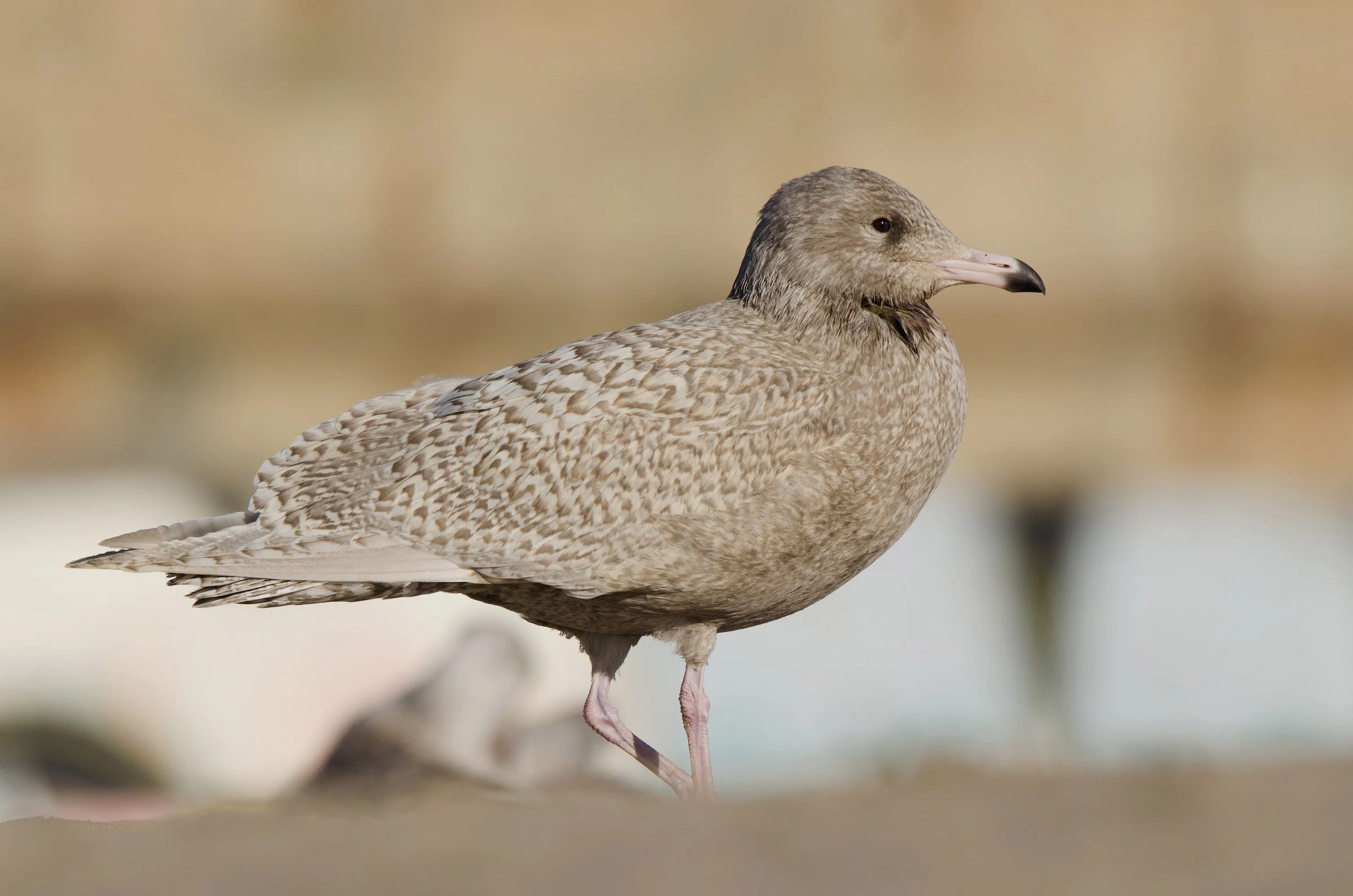
The cause of darker plumage in juvenile Glaucous Gulls, particularly in the hyperboreus ssp. wintering in Northern Europe, is not well understood, but it could feasibly have to do with historic hybridization with European Herring Gull (research suggests this happened a lot). Since darkly pigmented juveniles like this are frequent, it is likely that an individual Glaucous Gull can carry genetic variants for both dark juvenile plumage and pale adult plumage—meaning this bird could grow up to look like a typical pale Glaucous Gull. The answer to the question, “is this juvenile gull darker due to hybridization with Herring Gull?” could be yes, even if that hybridization occurred on a large scale in the distant past.
Of course, hybridization is just one possible explanation for why this gull is darker–the point is that hybridization in the distant past might still leave traces in juveniles, even while not being represented to the same degree in adults.

A very pale 2nd cycle Iceland Gull. 23 Jan 2025. Toronto, ON.
Whether this bird is more likely to have originated in Greenland or North America is a question involving, among other factors, the degree of gene flow between the ancestral lineages of present-day populations on each landmass. The fact that this bird is immature further complicates the matter, as selective pressures that might have contributed to divergence in adult plumages over time (e.g. mate selection) may not have equally affected immature plumages.
Consider the juvenile Herring Gull


The examples above, considered three different species and observed at widespread locations across North America, demonstrate some of the overlap found in juveniles of the Herring Gull complex. Should the Vega Gull here be labeled as such if it were encountered in the winter in Newfoundland, or on the Great Lakes? If enough traits line up in one direction, is there some tipping point where vagrancy is a better explanation for the observed traits than the other factors discussed above (e.g. recent or historic gene flow, incomplete lineage sorting)? Should that tipping point be entrusted to human experience with appearances if the above factors are not at all understood?
Other things that can destroy gull identification
I chose to focus on hybridization and gene flow in the previous sections, as these topics seem to be particularly relevant in gulls. There are a number of other reasons why unrelated lineages (e.g. Trash Bird and Mega Rarity) can show overlapping appearances. One is convergent evolution, where distantly related taxa evolve similar appearances without the existence of gene flow, maybe by being acted on by similar selective pressures. For example, distantly related species of gull might evolve a similar appearance if it helps them sneak up on surface-feeding fish from above. Another possible factor is phenotypic plasticity, where the appearance of an individual shows variation due to environmental factors within an individual’s lifetime. A classic example is the variable pink suffusion in certain bird species that is dependent on carotenoids in diet. Molt timing is another trait that likely is strongly influenced by short-term circumstances, like the availability of food, or whether or not an individual has chicks to feed that year. Considering that the redpoll complex shows an apparent smooth gradient of variation but has three discrete genotypes associated with this range of appearance, phenotypic plasticity may also be at play in some way.
The hybrid elephant in the room
One of the largest problems facing modern gull identification is the lack of understanding of appearances in hybrids and backcrosses. At present, identifying hybrids usually involves pointing to a gull and saying “that looks like one of those plus one of those.” To put this in more objective terms, if an individual shows a combination of traits that is extremely unlikely in any one species, but highly likely if you pool the traits of two particular species and include every intermediate, then hybrid parentage may be the most likely possibility. While there is a great deal understood when considering these “obvious” hybrids, it is problematic to assume these individuals represent the full range of variation in hybrids and especially backcrosses.
People tend to think of hybrids as if first-generation hybrids should look halfway intermediate between parent species, backcrosses should look progressively more like one parent species, and so on. There are a number of reasons why this is an oversimplification. As any pigeon breeder will tell you, trait dominance can drastically alter this picture. For example, if a “hybrid” trait (e.g. wingtip melanism in Glaucous Gulls) is associated with a dominant version of a gene, it can persist through any number of backcrosses with a parent species as long as those individuals only carry the recessive version of the gene. When traits are influenced by multiple genes, which is often the case, genes can have additive effects, or certain genes can regulate (turn “on” or “off”) the expression of others. The list goes on. In short, the contribution of one or the other parent species can be obscured or amplified depending on the specific combination of genetic variation inherited by an individual and so cannot be assumed based on appearance.

Source: Dittmann, D. L., and S. W. Cardiff. 2005. Origins and identification of Kelp × Herring Gull hybrids: The "Chandeleur" Gull.
The hybrids of Kelp and Herring Gulls on the Chandeleur Islands represent a rare case where researchers were able to observe the early stages and growth of a hybrid population. As the scale of hybrid pairs grew, any certainty the researchers had about what generation of hybrid or backcross they were looking at went out the window. The researchers explicitly acknowledged this: “…it was no longer possible to assume that an apparent F1 was really a true F1, as opposed to a second-generation (or higher) progeny of a pair of F1s or of some other backcross combination. Therefore, in the following discussion ‘F1’ refers to a general phenotype (F1s or hybrids that look more or less like F1s.)” From that point on, the authors refer to F1 and backcross “types” in the article. Sound familiar? They are not assuming genotypes based on phenotypes.
If the trait distributions of hybrids and backcrosses are unknown, then the degree of overlap that can occur is unknown.
Looking at the range of upperparts of the hybrids and backcrosses in the “Chandeleur” Gulls above, you may think this shows a clear-cut range for individuals with this hybrid ancestry. But remember that both Kelp Gulls and Herring Gulls have a range of upperparts themselves, and defining a boundary between “parent” and “hybrid” upperparts quickly leads to the same issues previously described in the section on gene flow and introgression. Such boundaries may emerge from the type of variation shown by certain traits, or they may not. Are there smooth gradients in the traits at the transitions between hybrid and parent types, or distinct clusters? Do phenotypes and genotypes vary in the same way? If parent and hybrid 'types' can be consistently defined as phenotypic categories, then their ranges, averages, and variance could be quantified—yet this kind of large-scale sampling has not been done for any hybrid gull.
Without these measures, one cannot know the degree to which Chandeleur hybrids or backcrosses (“hybrid types”) show overlap with Lesser Black-backed Gulls, whether in upperparts, bill size, leg color, or any number of traits. Cases of overlap may be extremely rare, or they may be so common that a significant proportion of hybrids are easily missed or not safely identified.

Possible Kelp x American Herring Gull hybrid type. 20 April 2024. TX, US.
On close inspection, this individual shows some traits that are highly unlikely in Lesser Black-backed Gull, such as a yellow-orange orbital ring. A number of traits line up with descriptions of Kelp x American Herring hybrid types (“Chandeleur” Gulls). The individual it associated with, another suspected Chandeleur-hybrid type, showed a bill so large that it was assumed to be outside of range for Lesser Black-backed Gull based on experience. Without that more obvious individual, this bird could have easily been overlooked due to extensive overlap in appearance with Lesser Black-backed Gull.

Possible European Herring Gull x Glaucous Gull hybrid type. 04 Aug 2024. Reykjavik, Iceland.
This individual shows a bill and head that are small even for a Herring Gull, and put it within the range of the Iceland Gull complex. Certain plumage characteristics may be unlikely in an Iceland Gull, but are they diagnostically outside of range? Compare the pattern on the primary tips to 32c.9, p.421 of The Gull Guide, for example. The date and location of this sighting weigh heavily on the likely origins of this individual.
These two examples highlight how the uncertain distributions of traits in hybrids can lead to an unknown degree of overlap. In many cases, one is left asking “is this a typical individual of an extremely unlikely kind, or an extremely unlikely individual of a typical kind?” This is the Perfect Vagrant scenario all over again. The degree of overlap in hybrids and backcrosses will remain unknown until there are studies with representative samples of gulls that have known hybrid ancestry.
Glaucous-winged Gulls complicate these matters considerably, as their various hybrid pairings open the potential for transfer of genes between a minimum of five different species, two of which are known to hybridize themselves (Glaucous Gull and American Herring Gull). While these pairings occur at drastically different frequencies, with hybrids of Western and Herring Gulls being the most numerous, it is entirely possible that gene flow between more than two species has occurred in the recent past or is ongoing. This means that a single individual could conceivably show traits that evolved separately in three, or even more, distinct species. This may seem like some fairy tale nightmare specifically designed to torture birdwatchers, but it is a real possibility, and especially so in immatures. Remember that hybridization can happen over many generations, on and off over tens of thousands of years, and genetic research to date has only shown support for extensive hybridization in the evolutionary history of large white-headed gulls.
Taking this all in, the extent of uncertainty regarding ancestry on the Pacific coast is overwhelming. Questions like 'Is this juvenile a Glaucous-winged × Herring hybrid, or a Glaucous-winged × Western hybrid?' seem, to me, to be missing the magnitude of the utter mess involved. How is Glaucous Gull ruled out as a possible contributor to an uncommonly pale Herring type? What about Slaty-backed Gull? Just because individuals from these species are uncommon at a given location, doesn’t mean their genetic variation is equally rare there—especially if gene flow has already incorporated it into the broader gene pool. Consider that the genetic contribution from another species could emerge at any point in the untold number of mate pairings in an individual’s ancestry and could persist for any number of generations. It is possible that gene flow is restricted to hybrid zones and does not lead to Frankenstein juveniles with traits of five different species, but this is an assumption (maybe a secret hope) and is not based on any real knowledge of gene flow in these populations.

Glaucous-winged Gull. 17 Nov 2018. British Columbia, Canada. Photo credit: Blair Dudeck.
The Glaucous-winged Gull (Larus glaucescens) is known to hybridize with at least four species, two of which also hybridize with each other. Large-scale hybridization with Western Gull and American Herring Gull contributes to a gene pool influenced by at least three species. The extent to which gene flow is restricted to discrete hybrid zones remains uncertain. The only genetic research on the subject, focusing at the “Olympic Gull” hybrid complex, was published in 1996 and analyzed only 32 genetic loci. Compare this, for example, to the recent research on the flicker complex that required whole-genome sequencing and millions of genetic variants.
Q: Where do we go from here?
A: Observe traits, try not to make assumptions about genetics.
If you see a bird that looks like an adult Slaty-backed Gull in North America, then it’s fair to assume that bird was born in Asia, or somewhere very recent in its ancestry are birds that were born in Asia. If you see something that looks like a juvenile Slaty-backed Gull–where some individuals may have complete overlap in appearance with a number of expected North American taxa–then assuming it was born in Asia means assuming that its traits are not the result of gene flow (recent or distant), retained ancestral variation, or some other mechanism that creates overlap. If you’re comfortable drawing these conclusions, that’s fine, but you should at least be aware of what the range of possibilities are. If you are not so sure, then the more cautious route is simply to note what you are sure of:
1) the traits you observe, and
2) where and when you observe them.
This could mean documenting your observations more precisely, using subspecies, 'slash' notations, or hybrid labels on eBird. You can also keep track of individuals with unusual trait combinations that don’t fit within existing labels. If you want to take it further, you can use a spreadsheet to score traits from multiple individuals and analyze patterns statistically. Patterns in phenotype and geography could hint at underlying patterns in genetics, or they might not. They could offer insights into vagrancy, hybridization, or even the evolutionary history of species not known to hybridize. Or the patterns you find could relate to some environmental influence that acts independently of genetics.
Looking back at the flicker, warbler, and redpoll complexes discussed earlier, it was only after observers first established a clear picture of phenotypic variation that researchers could determine how genetic differences related to appearance–including whether groups should be considered distinct species, subspecies, or types.
Gulls will continue to challenge our attempts to fit them into well-defined categories. Individuals that suggest vagrancy or hybrid ancestry provide opportunities to refine our understanding, but only if we recognize the limits of what we can observe.